 |
Maxwell Viscoelastic Fluid | Maxwell Legacy Concepts |
|---|
In a nutshell |
All fluids in everyday life have viscosity, both liquids and gases. Clear honey is more viscous than water, water more viscous than alcohol; cold water about twice as viscous as hot water. Engine oil is specifically sold in various grades corresponding to its viscosity. Viscosity affects how quickly liquids flow in a given circumstance. Viscosity is a form of internal friction and as such during flow results in energy dissipation as heat. Viscosity of the atmosphere causes sounds to fade out more quickly in the open than the inverse square law predicts. Without the viscosity of air, most professional golfers and good amateurs would be able to drive a ball half a kilometre. Materials that obey the usual rules of viscosity are called Newtonian. Elasticity is the basic property of springs. In the days when clocks were purely mechanical, watches, chronometers and travelling clocks all had springs; almost all vehicles have springs, in their suspension or engine, or both. In the house, springs are found in all sorts of items from beds through door handles to clothes-pegs. A useful property of a spring is that the energy taken to stretch it is recovered when the spring contracts. Some springs work in compression rather than extension, but the physics is the same. It was Robert Hooke in the 1670s who first quantified how springiness worked. He found that the restoring force was directly in proportion to the extension of the spring. The more a spring is stretched (or compressed), the harder it pulls (or pushes) back. Maxwell's entry in the field wasn't motivated by any investigation into quirky springs or quirky viscosity. He was investigating from first principles the properties of gases in particular and at times fluids in general in a treatise length paper of 1866. He considered a model of fluid flow that was in essence a spring in series with viscous drag. The applied stress was felt by both components; the response was the sum of the responses of both. A fluid whose flow properties can be modelled like this, or in a similar way, is called a Maxwell fluid. It behaves partly like a spring and partly like a viscous liquid, summarised in the description viscoelastic. One distinctive property of a viscoelastic fluid is that if the stress is removed quickly, the strain doesn't disappear at once but relaxes, perhaps quite slowly. Polymer fluids and a good many naturally ocurring materials are viscoelastic. Another behaviour is that if a stress is applied and maintained, the viscoelastic material responds quickly and then creeps to a greater strain. One example of viscoelastic behaviour is the phenomenon of our daily shrinking in height. Upon getting up in the morning the discs in our spine are suddenly loaded. Over the day the response creeps up and the discs shrink slightly under the continued weight. By the evening we are measurably less tall. Another feature of a viscoelastic material is that it shows hysteresis when a cyclic load is applied. The strain change on applying a load is not the same as the change on removing the load. There is a net amount of work done if a load is applied and then removed. In other words, the energy expended in stretching a viscoelastic material is not all recovered when the material contracts. Not all viscoelastic materials are Maxwell fluids, for some exhibit more complex properties than those given by Maxwell's comparatively simple model. Nonetheless, Maxwell was the first to model a non-Newtonian fluid. |
 A pendant drop of a Maxwell fluid breaking up, illustrated in H. Tabuteau, et al, Propagation of a brittle fracture in a viscoelastic fluid, Soft Matter, 2011, 7, pp 9474-9483. A pendant drop of a Maxwell fluid breaking up, illustrated in H. Tabuteau, et al, Propagation of a brittle fracture in a viscoelastic fluid, Soft Matter, 2011, 7, pp 9474-9483. |
|---|
| Technical detail |
Viscosity is determined by thinking of two planes parallel to the local flow separated by a small distance dz. Fluid on the two planes will be travelling at different speeds (difference du) and the slower one will exert a retarding shear on the faster one. For a Newtonian fluid, the force per unit area is proportional to the velocity gradient perpendicular to the flow: f =η du/dz. η is the viscosity. Maxwell was very comfortable with the theory of elasticity, having written while still a teenager a lengthy paper On the equilibrium of elastic solids that was published in the Transactions of the Royal Society of Edinburgh. In Maxwell's take on fluid flow, the viscosity shown by a fluid is the end result of the rigidity of a solid breaking down under shear stress. If the planes mentioned above are travelling in the x direction with the faster one travelling an extra distance dx in a short time dt, then the rigidity μ is defined from the relationship f = μ(dx/dz). As the shear displacement gets greater it breaks down and reforms with a time constant of τ. The rate of change of the shear is d/dt.(dx/dz) = du/dz = (dx/dz)/τ. The net result of this model is that f/(τ μ) = f/η. Hence τ = η/μ. This makes sense, for if the time constant is long then the viscosity is large or the rigidity modulus small, or both. Taking the matter further, in Maxwell’s day both he and his contemporaries tended to explain the unknown in terms of conceptual mechanical models. Today we are more likely to explain mechanical systems in terms of electrical systems. An exact analogy can be made, and Maxwell did like analogies, between voltage, current, resistance, capacitance and inductance on the electrical side and force, velocity, dashpot, spring and mass on the mechanical side. Mechanical systems can be represented by ‘lumped components’ in an analogous way to circuit diagrams. Indeed, Maxwell is credited with being the first to use the ‘impedance analogy’, though in his case he was explaining electrical phenomena in terms of the mechanical. The method was taken a long way in mid 20th century with the construction of analogue computers that simulated complex mechanical systems. This preamble is relevant to the first figure on the immediate right that is often drawn to represent a simple Maxwell fluid by a dashpot and spring in series. Below is an equivalent electrical circuit. In the electrical circuit, the resistor and capacitor together create the time constant τ = RC where the capacitance C is proportional to the inverse of the spring constant μ. The current represents the velocity of the system and hence the strain is represented by the integral of the current, shown by the blue curve in the lower figure over 3 time constants once the load (voltage) is applied. The curvature represents the time for a loaded system to head towards equilibrium, i.e. the creep in a viscoelastic system. The resistor absorbs power in a cycle, representing mechanical hysteresis. The brown curve shows the result of the voltage being set to zero for 3 time constants, equivalent to removing the load. The capacitor discharges and the system relaxes. [With time increasing, the brown curve should really be extended to the right from 3 to 6 time constants but has been drawn to the left to emphasise the similarity to a hysteresis curve].
JSR 2016 |
Top: mechanical representation of a simple Maxwell fluid. Bottom: electrical analogue.
|
|---|
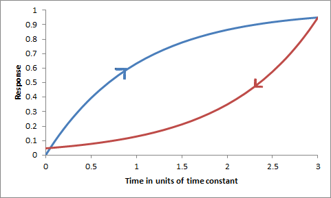 Electrical analog with voltage applied for 3 time constants (blue curve) representing loading (illustrating mechanical creep) and system discharging for 3 time constants (brown curve) representing relaxation.